ACM Transactions on Graphics · 2026
Best papers award honorable mention
Sample Matching for Joint Extinction Gradient
Estimation in Differentiable Volume Rendering
1The University of Tokyo 2Tsinghua University 3University of California, Irvine 4University of Illinois Urbana-Champaign
TL;DR
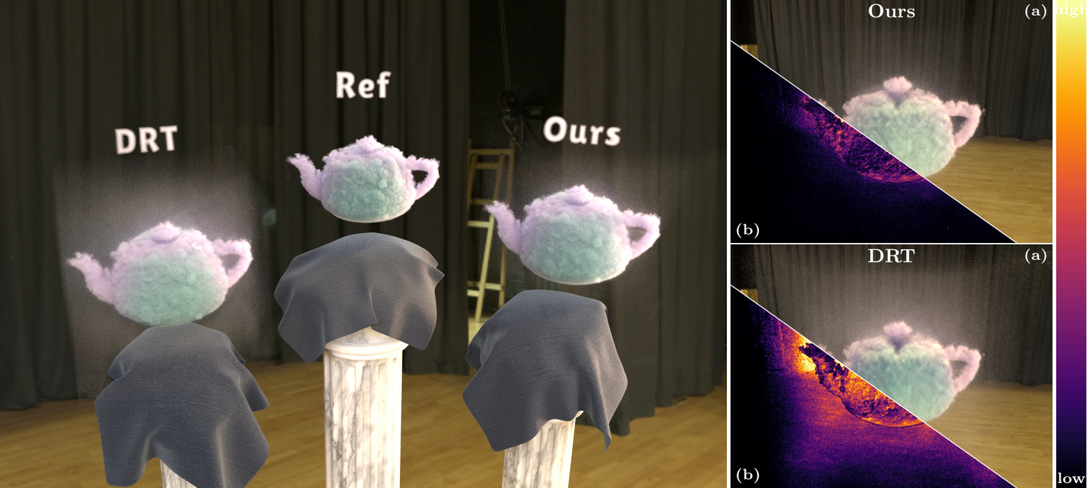
We model the extinction (or, plainly, density) gradient as the difference between the in-scattering radiances of two paths. That mirrors what the physics is doing: increasing density at a point adds in-scattering and attenuates background transmission, so the gradient is naturally the sum of two terms with opposite signs.
Existing unbiased estimators never couple these two terms — they evaluate the scattering and transmittance contributions at different points along the segment, so the cancellation that should reduce variance becomes pure noise instead.
Coupling them is non-trivial because the two terms live on different integration domains. A short derivation built on Fubini's theorem and the definition of transmittance is enough to put both terms on a shared domain, so they can be evaluated at the same probe. Once they share a sample location, their opposite-sign correlation collapses much of the variance.
In practice this is a near drop-in: even without the most-tuned codepath, a handful of lines on top of an existing volumetric path-integral estimator already yields a large variance reduction.
Why two opposite-sign terms?
Nudging the medium denser at one point does two things at once: it blocks more of the red, in-line background radiance the camera was already seeing, and it scatters more of the blue, off-axis radiance into the same outgoing ray. The density gradient is the difference between the two radiances. Drag \(\sigma_t\) below to watch the trade-off.
Where does the scattering probe land?
The three estimators agree on the transmittance probe (uniform on the host segment) and only differ in where the scattering term reads \(\partial\sigma_t\). Each schematic shows two lines on the same axis: the top one is the scattering probe with its sampling PDF drawn as a blue silhouette; the bottom one is the transmittance probe. DRT's scattering PDF lives on the segment extended to the medium boundary \(x_j^{\bot}\) (violet dashed).
Video
BibTeX
@article{yu2026samplematching,
  title     = {Sample Matching for Joint Extinction Gradient Estimation in Differentiable Volume Rendering},
  author    = {Yu, Ruihan and Wang, Yu-Chen and Ling, Jingwang and Xu, Feng and Zhao, Shuang},
  journal   = {ACM Transactions on Graphics},
  year      = {2026},
  month     = jul,
  volume    = {45},
  number    = {4},
  articleno = {136},
  numpages  = {15},
  doi       = {10.1145/3811329},
  url       = {https://doi.org/10.1145/3811329},
  publisher = {Association for Computing Machinery},
  address   = {New York, NY, USA}
}